Advanced Tables and Charts in Excel with Simple Steps
Charts, pictures, and boxes are great ways to visualize and represent data, and Excel is capable of creating them automatically. There may be times when we want to go beyond the basic charts that Excel creates for us. In this simple guide, we will focus on this complexity so that you can create advanced charts in Excel.
What are Advanced Charts in Excel?
An advanced chart in Excel is a chart that goes beyond the basic charts created by Excel by default. Suppose you have more than one data set that you want to compare on the same chart. You can create your basic chart with one dataset and then add other datasets to it and apply other elements i.e. format the chart. This is what advanced graphics are.
What do advanced charts offer us?
- They provide consolidated information in a single table, making it easy to compare multiple data sets, allowing you to make quick decisions.
- They allow us to customize the appearance of the graphics.
Step by step tutorial to create an advanced chart in Excel
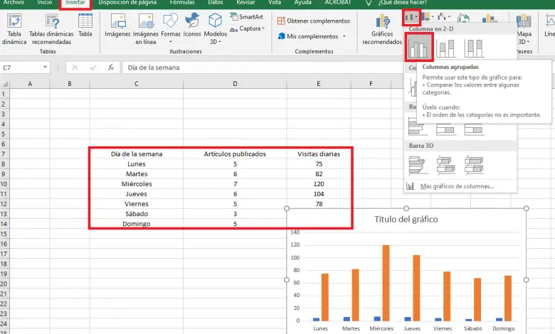
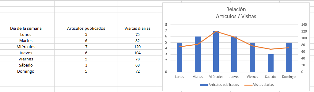
In this example tutorial, we'll assume that we have a webpage and web traffic control that gives us the number of daily visits. With this data, we would like to see the relationship between the number of articles we publish per day and the total daily traffic. We will work with the following dataset.
| Day of the week | Published articles | Daily visits |
| Monday | 5 | 75 |
| Tuesday | 6 | 82 |
| Wednesday | Sept | 120 |
| Thursday | 6 | 104 |
| Friday | 5 | 78 |
| Saturday | 3 | 68 |
| Sunday | 5 | 72 |
You can also use other data, such as a relationship between income and expenditure in the months of the year .
For this example, create a new worksheet in Excel and copy the data above. Then select all the cells that contain the data (without the headers) and go to the "Insert" tab and select the bar charts option.
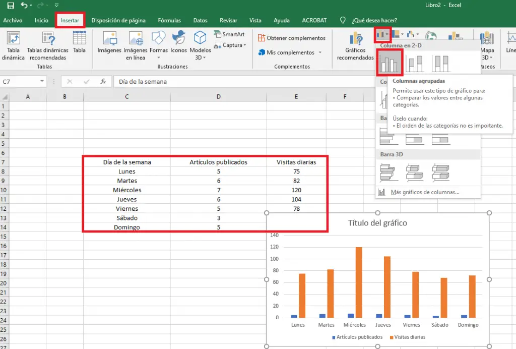
With this we already have our basic chart with the data from the table. We will now continue to push this graph a little further.
Select one of the bars in the graph. For example an orange. Now go to the "Design" tab and select "Change chart type".
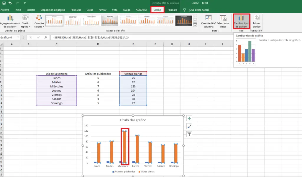
In the window that will open, select the “Combined” option in the left menu, then change the data type of daily visits to “Lines” and check the “Secondary axis” box.
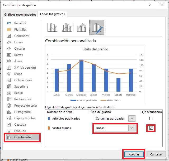
Congratulations, you have just created an advanced chart that combines two types of charts separated by two axes.
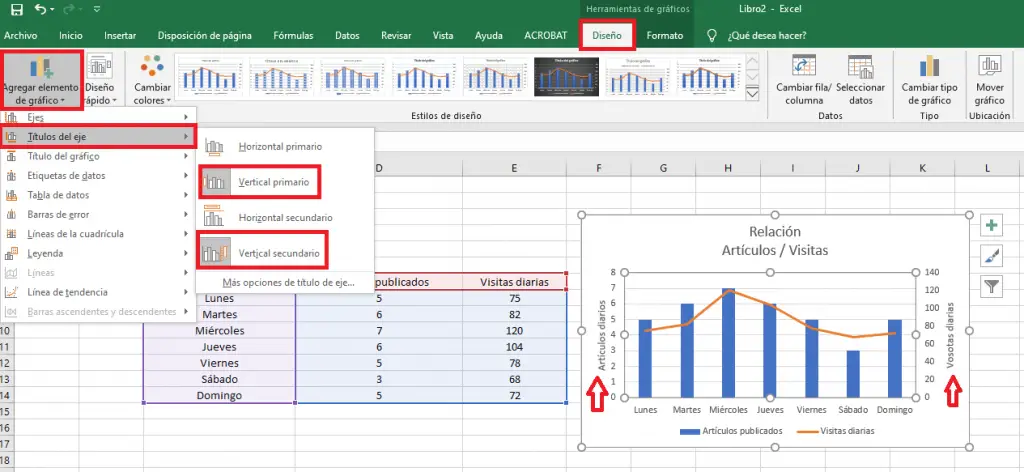
Finally, you can edit the chart by changing the main title, as well as add the titles of the primary and secondary axes by going to the “Design” tab, selecting “Add a graphic element” then under “Axis title "Click on" Primary vertical "And" Secondary vertical ".
The steps are very simple and quick. Of course, you can modify more options of the graph by adapting it to your needs in the window "Design" -> "Change the type of graph" -> options of the left menu.
If you found it interesting, find out now how to lock cells so that they cannot be edited or deleted .